Introduction to Projections - Part 2

Week 5 – Projections Part 2

For this week’s assignment, we continued working with map projections in ArcMap. In addition, we also downloaded shapefile and aerial images from different websites. Land Boundary Information System (LABINS) and Florida Geographic Data Library (FGDL). We also had to create an Excel spreadsheet with Latitudes and Longitudes in Degrees, Minutes, and Seconds. After that we had to format them in Excel, and then convert the information to Decimal Degrees and format in Excel once again. 

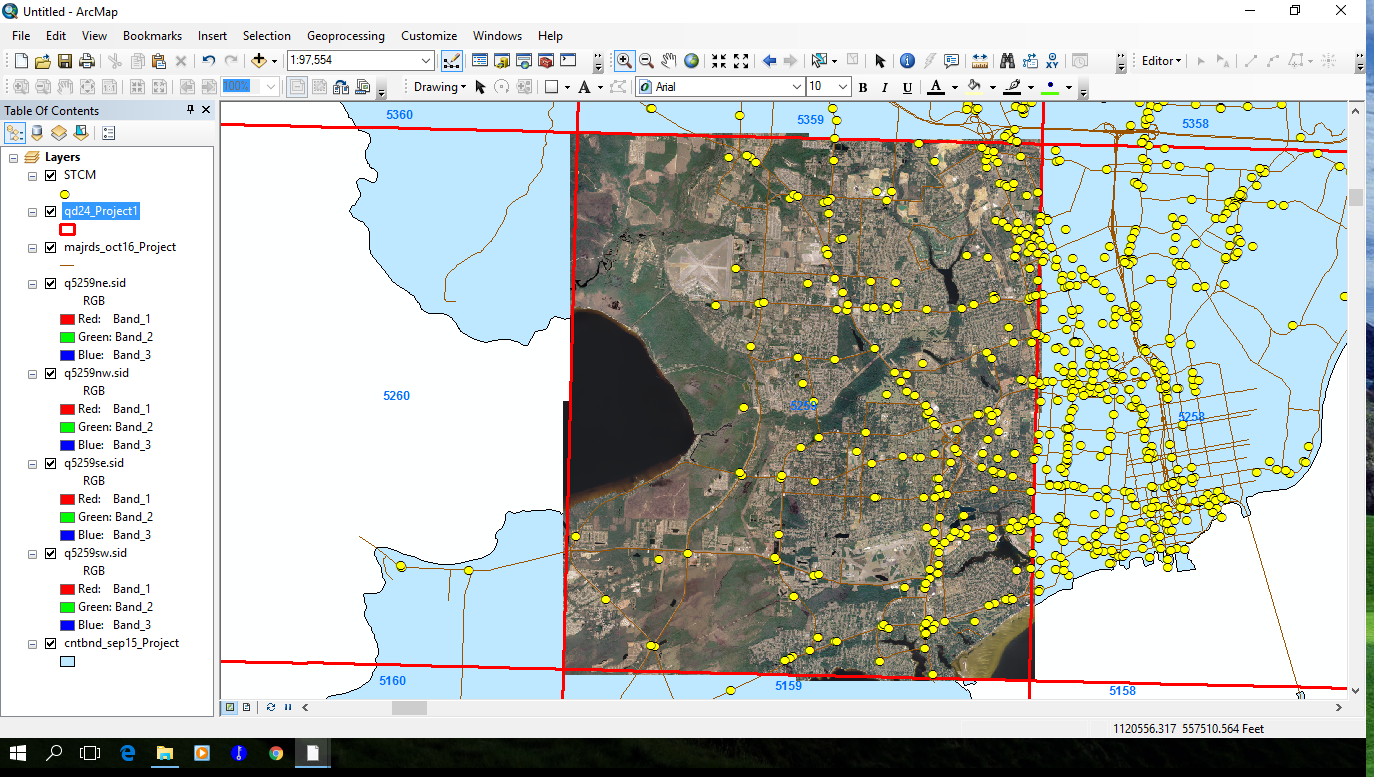
Using some of the data we downloaded, we had to re-project the data to the coordinate system that we were using. The other data we had to define the projection so it lineup correctly with the other information.

For the Excel spreadsheet we had to convert the Latitudes and Longitudes from Degrees, Minutes, and Seconds, to Decimal Degrees.  Then you were able to add the spreadsheet date to ArcMap to give you point features for the locations. 

This was a long lab assignment but a very good one. This has helped me immensely to understand in depth, about projections and how to use them. 

Introduction to Projections

Week 5 – Projections Part 1

For this week’s assignment we learned about map projections and how they work. As part of our lab assignment we were asked to show three different projections side by side:  Albers, UTM and State Plane.  We were also asked to highlight four counties in Florida. The counties were Alachua, Escambia, Miami-Dade and Polk. We were asked to show the projection comparison by area in square miles for each county.

Albers Equal Area Conic: Is used by the US Geological Survey (USGS) for maps of the conterminous United States.

UTM: Universal Transverse Mercator is one of the most used map projections; mainly used for rectifying remotely sensed data and large scale topographic mapping.

State Plane:  These are individual state’s projections; they are based on the state’s shape and geographic location.

Sharing GIS Maps and Data

Week 4 – Sharing GIS Maps and Data

For this week’s assignment we were asked to come up with a Top 10 List of some of cities I have visited over the years.  We used Excel to rank the list and then we added the address, zip code, and the state. We were also asked to add the URL address, which is the website address.  I used each city's City Hall website for my list.  We also used ArcGIS online and Google Earth to show the locations of the cities for the list.

ArcGIS online allows you to make maps online and have the ability to share them with the public if you choose to. In addition, with ArcGIS online we were also able to Geocode the address for the top 10 list, and showed the locations on a map. 

My ArcGIS Map:    http://arcg.is/2kQONnn

For Google Earth we used ArcMap to make a KMZ file. This is a place marker that can have some data attached with it.  It’s an easy way to share information with others. This allows them to see the location and click on it to see the attached data.

GIS Cartography

Week 3 – GIS Cartography

For this week’s assignment we learned more associated tools in ArcMap and we also learned how to add graduated colors to make a population map of Mexico.  The graduated colors help to see areas that are more populated from than areas that are not.  We also made a map showing the rivers, railroad tracks, and federal roads, and the urban area in Mexico.  The third map was a topography map of Mexico. This map helps you understand the high and low regions of the areas of Mexico. I liked making this map. The most I like was going through the color ramp and trying to find the best color for your audience to understand your map.